The Fundamental Plane of Black Hole Accretion and Its Use as a Black Hole-Mass Estimator
; King, Ashley L.; Cackett, Edward M.; et al.
The Astrophysical Journal, Volume 871, Issue 1, article id. 80, 23 pp. (2019).
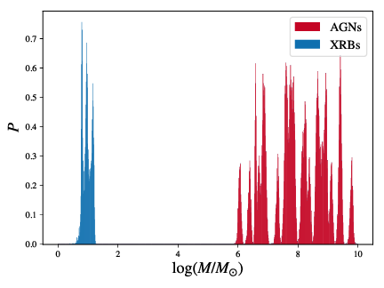
COMBH2 MBH Histogram
Probability density of black hole masses for the entire sample. We plot multiple realizations of our sample from the masses with uncertainties and their dependence on distance for the AGN sample. Thus, the distribution of the probability density of an individual black hole's mass combines the statistical measurement uncertainties of both the mass and the distance. We do not include distance uncertainty in the XRB mass probability density because it generally does not affect it. The range of masses included in our sample is illustrated in this figure.
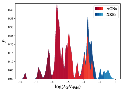
COMBH2 fedd plot
Probability density of logarithmic 2–10 keV X-ray Eddington fraction. We plot multiple realizations of our sample using statistical uncertainties of X-ray flux, distance to source, and black hole mass. For AGN sources, we take into account the correlation between distance in the luminosity calculation and distance in the mass estimate. The multiple observations of individual XRBs are incorporated by weighting each as 1/N, where N is the number of observations of a given XRB. The probability density curves are colored according to mass category (red for AGNs and blue for XRBs) and the shade is given by the value of $mathrm{log}({L}_{X}/{L}_{mathrm{Edd}})$. AGNs are grouped into the following discrete bins: $(-infty ,-8)$, [−8, −6), [−6, −4), and $[-4,+infty )$. XRBs are grouped into the following discrete bins: $(-infty ,-2.5)$, [−2.5, −1.5), [−1.5, −0.5), and $[-0.5,+infty )$. We use this color scheme in figures throughout this paper. Note that the probability density plotted is the total probability density of all sources so that at, e.g., $mathrm{log}({L}_{X}/{L}_{mathrm{Edd}})=-4,$ the probability density is dominated by AGNs with a small contribution coming from XRBs. The nearly 10 orders of magnitude in X-ray Eddington fraction covered by our sample is illustrated in this figure.
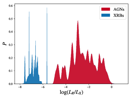
COMBH2 L_R / L_X hisogram
Probability density of the logarithmic ratio of radio to X-ray luminosity. We plot multiple realizations of our sample using statistical uncertainties of radio flux and X-ray flux. As in the rest of this paper, radio "luminosity" is defined as LR ≡ νLν for ν = 5 GHz, whereas the X-ray luminosity is a true 2–10 keV bandpass luminosity. The uncertainty in the radio luminosity also incorporates our estimate of systematic uncertainty in converting from other frequencies to 5 GHz. The nearly 8 orders of magnitude probed by our sample is illustrated in this figure as is the larger fractional uncertainties in the AGNs.
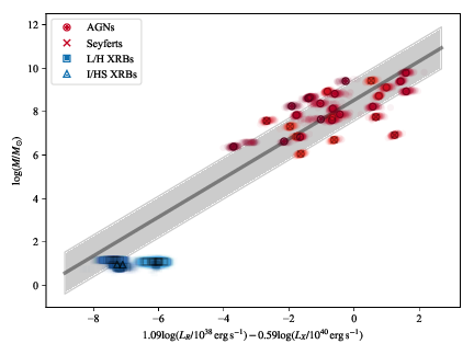
COMBH2 Edge-on
Edge-on view of the fundamental plane with mass as dependent variable. Here we plot all data realized N times to show the correlated uncertainties. Colors are as in Figure 2, and symbols indicate whether the source is an AGN (red circles), a Seyfert AGN (red circle with cross), an XRB in a low/hard state (blue squares), or an XRB in an intermediate or high/soft state (blue triangles). Each source is sampled from its measurement uncertainties as is done in the fitting procedure and is plotted with a partially transparent symbol plus a dark outline symbol on top at the nominal values. We plot the best-fit relation as a dark gray line with a light gray shaded region to indicate the 1σ region of the Gaussian intrinsic scatter, which has magnitude of 1 dex. This figure summarizes the results of the fits as well as indicates the fidelity with which one can use the fundamental plane to estimate black hole mass.
COMBH2 Corner Plot
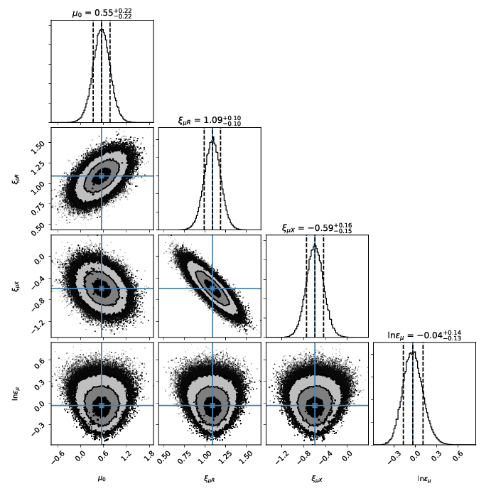
A Foreman-Mackey (2016) corner plot of MCMC results. Each panel in this corner plot of our MCMC results shows either the posterior probability distribution of an individual parameter in our fits (histograms) or the joint posterior probability distribution of pairs of parameters (scatter plots). The equations at the top of each column show the median and 68% interval of each parameter, μ0 = 0.55 ± 0.22, ξμR = 1.09 ± 0.10, ${xi }_{mu X}=-{0.59}_{-0.15}^{+0.16}$, and $mathrm{ln}{epsilon }_{mu }=-{0.04}_{-0.13}^{+0.14}$. The posterior distributions show well-behaved, mono-modal distributions. The joint posterior distributions show some covariance between ξμR and ξμX as well as between μ0 and either of ξμR and ξμX. The asymmetry in the joint posterior distributions that include $mathrm{ln}{epsilon }_{mu }$ is typical when using a logarithmic intrinsic scatter term. For comparison, the corresponding fits from Gültekin et al. (2009a) are μ0 = 0.19 ± 0.19, ξμR = 0.48 ± 0.16, ξμX = −0.24 ± 0.15, and $mathrm{ln}{epsilon }_{mu }=-0.26$.
COMBH2 N4459 radio map
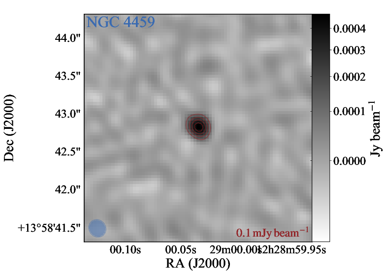
Example of our VLA maps using NGC 4459. Full figure caption is: VLA maps of our new 8.4 GHz X-band observations of 12 sources. Grayscale is indicated by the bar to the right of each panel, and the contours are in constant steps of the value indicated in the lower-right corner of each panel. The blue ellipse in the lower-right corner of each panel shows the size and position angle of the synthesized beam. The maps are centered on the brightest pixel within a 20 × 20 pixel region centered on the Simbad coordinates for the host galaxy. When the source is securely detected, it is always consistent with a point source. We list the integrated flux densities and upper limits in Table 1.
A comprehensive look at X-ray and radio emission from black holes with dynamically measured masses and how it can be used to estimate black hole mass. Also check out the 3D interactive visualization (not sure why it isn’t on the ApJ page right now now on the ApJ page).